Smoothing¶

Introduction¶

Smoothings generate a new set of data points from the existing dataset. In CurveExpert Pro, Lowess smoothing is supported, as well as moving averages with an averaging window defined by the user.

Lowess Smoothing¶

To calculate a Lowess smoothing, select Calculate->Lowess Smoothing from the main menu. Lowess smoothing (which stands for LOcally WEighted Scatterplot Smoothing) builds on regular linear regression in order to smooth an existing dataset; in this context, an entirely new dataset will be generated that represents the smoothed data. Lowess smoothing generates a polynomial fit to a subset of data around each point in the dataset. More weighting is given to points near the point of interest, and less weight is given to points far away. After the polynomial is determined, a “smoothed” y data value is obtain by evaluating the polynomial at x.

The weighting function used is the tri-cube weighting function for $|x| < 1$ :

$w(x) = \left (1 - |x|^3 \right )^3$

where $x=(x_i - x_p)/s$ , and the weighting function is zero for $|x| >= 1$ . $x_p$ is the point of interest, and $s$ is the maximum distance of any point in the local dataset to $x_p$ .

The polynomial used by CurveExpert Pro is a simple degree-one linear regression. Once the smoothed values are obtained, a linear spline is used to connect the points for visualization and evaluation purposes.

Note

William S. Cleveland: “Robust locally weighted regression and smoothing scatterplots”, Journal of the American Statistical Association, December 1979, volume 74, number 368, pp. 829-836.

Note

William S. Cleveland and Susan J. Devlin: “Locally weighted regression: An approach to regression analysis by local fitting”, Journal of the American Statistical Association, September 1988, volume 83, number 403, pp. 596-610.

Savitzky-Golay Smoothing¶

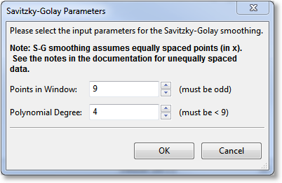
To calculate a Savitzky-Golay smoothing, select Calculate->Savitzky-Golay Smoothing from the main menu. Savitzky-Golay (SG) smoothing combines a moving-average-type averaging with a locally-fitted polynomial in order to smooth an existing dataset. The user has the opportunity to select the number of points in the moving average window (the number of points must be odd), and the degree of the polynomial used to fit the data within each window. Additionally, the degree of the The input dialog for the SG parameters is shown below.

SG smoothing is primarily intended for data that is equally spaced in x (typically, x is time). In cases where the x data is not equally spaced, CurveExpert Pro still assumes that it is for the purposes of performing the smoothing. Doing so virtually shifts the data points to equally spaced positions within the averaging window. In cases where smoothing is useful in general, this shift is the equivalent of introducing an additional source of noise in the function values; however, this noise will often be much smaller than the noise already present in the samples. Thus, the smoothing is still useful, but should be used with care. The nature of smoothing in general is just to guide the eye through a forest of points, so the user can determine if the output smoothing performs its desired task rather easily.

Moving Averages¶

Moving average applies an averaging window to each point in a dataset, in turn, in order to generate a new set of data. The size and type of window determine the amount of averaging that will take place. To calculate a moving average, select Calculate->Moving Average from the main menu. A dialog will appear that will allow you to select the window to utilize for the averaging.

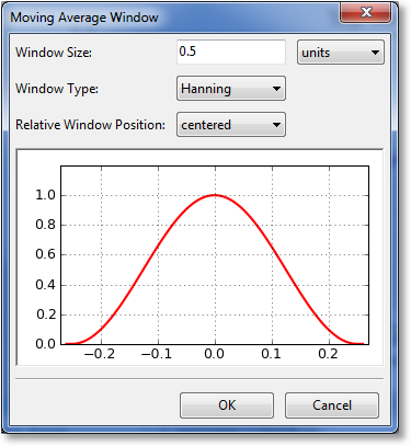
The first parameter to select for the window is its size. Here, you can select the size (sometimes called the extent) of the window in terms of units (meaning a distance along the x axis), or in terms of number of points. The (0.0) location on the preview is always defined to be at the x location of the point being window averaged. The window preview will continually update in order to show the currently defined window. Note that the underlying dataset must be sorted in order for the window to be specified in terms of a number of points. If the dataset is not sorted, the points choice is disabled.

The window type can also be selected from the following:

rectangular
Bartlett (triangular)
Blackman
Hamming
Hanning

The window type affects the weighting factor that is applied to each point within the window that is to be averaged. For example, a rectangular window applies a weight of 1 to all points within the window.

Finally, the relative window position can be set. Usually, a centered window is used, which places the center of the window at the same x location as the data point being averaged (location 0.0). Alternatively, you can select a leading or lagging window, which places the window ahead of the data point or behind the data point, respectively.

After tuning the window parameters to the desired settings, click “OK”, and the moving average will compute and display.