Calculating Results¶

CurveExpert Professional supports four distinct classes of results:

regressions
- linear regressions (linear and polynomial fits)
- nonlinear regressions (built-in and custom models)
interpolations
- linear spline
- cubic spline
- polynomial spline
- tension spline
smoothings
- lowess smoothing
- moving averages
functions (built-in and custom functions)

Calculation of these results can be accessed through the Calculate menu in CurveExpert Professional, or optionally via the corresponding buttons on the toolbar (see Toolbar).

Note

A distinction is made between “models” and “functions”. Models have free parameters, and are therefore dependent on the independent variables and the parameters: $f \left ( \vec x; \vec a \right )$ . Functions are dependent on the independent variables only, with no free parameters: $f \left ( \vec x \right )$ .

General Guidelines¶

Scaling Datasets¶

For best results, always scale your data sets to the order of one. You may do this prior to reading in your data file, or after your data file has been imported using the scaling feature in CurveExpert Professional (see Operating on Data).

Imagine a data set with x values ranging from 1000 to 10000 and a regression model where the term exp(a*x) is involved. Unless a very good initial guess for a is given, chances are that an exponential to a very large power (eg. exp(1000)) will be taken in the course of the nonlinear regression algorithm. The calculation will overflow, and the regression will fail as a result. Even if the regression happens not to fail, the regression algorithm will have an exceedingly tough time finding the correct parameters, since a small change in the free parameters will cause a tremendous change in the size of the term. The moral of the story: always scale your data!

As another example, if you have data that describes atmospheric pressure at different elevations, you might have (in metric units) a data set that looks like:

x=[-100, 0, 100, 500, 1000, 4000] meters
y=[102000,101325,101000,100500,100000,99900] Pascals

Using the Data->Scale feature in the Data menu of CurveExpert Professional, you can scale this data using a scale factor of 0.001 on the x data, and 0.00001 on the y data. So, you would then have the following data set:

x=[-0.1, 0, 0.1, 0.500, 1, 4] kilometers
y=[1.02,1.01325,1.01,1.005,1.0,0.999] bars

The second example is much more likely to allow nonlinear regressions to converge, and also will allow higher order polynomial fits to be performed with more accuracy. If you have a data set that seems particularly ill-behaved, scaling can help solve this problem.

Note that CurveExpert Professional is able to perform correctly on data in any scale, as long as the calculations do not overflow or underflow. So, if a data set is giving problems, scaling it should be the first action to take.

Weighting¶

Weighting has to do with defining how “important” a particular point is in the optimization calculation; i.e., accounting for the fact that in some cases, certain data in the dataset is more precise than other data. Thus, a greater importance should be placed on the more precise points. More precisely defined points (those with less uncertainty) should be given greater influence (a greater weighting) over the final fitted parameters.

There are six choices for weighting in CurveExpert Professional:

Default: No weighting unless a standard deviation column is defined in the dataset; in that case, weight by the square of the standard deviation column. This is equivalent to weighting by the uncertainty (if available).
None: No weighting under any circumstance, even if a standard deviation column is present.
Y: Weight each data point by the absolute value of its Y (dependent variable) value.
Y^2: Weight each data point by the square of its Y (dependent variable) value.
X: Weight each data point by the absolute value of its X (independent variable) value.
X^2: Weight each data point by the square of its X (independent variable) value.

Note that if there is more than one independent variable, weighting by X and X^2 will not be available.

Set the tolerance parameter reasonably¶

Don’t set the tolerance parameter (in Edit->Preferences->Regression) too low. In regression modeling, not much advantage is to be gained by setting a very strict tolerance. Its main purpose in life is to prevent the nonlinear regression algorithm from converging on local minima, not to make the calculated parameters more accurate.

Data should be appropriate to the model¶

Make sure that the data is appropriate to the model. Especially look out for using logarithmic or exponential families of models with data that contains zeros or negatives. For example, it is not possible, in any shape or form, to obtain a negative or zero with the basic exponential model (y=ae^(bx), assuming a is positive; the inverse problem exists for a negative a). So, it is not wise to use a model that cannot reflect the trends in the data.

For interpolations, data points must be sorted¶

If you are using an interpolation-type curve fit, the data points must be sorted by ascending x. Use the Data->Sort feature in CurveExpert Professional to sort your data points correctly.

Sometimes, it is unavoidable¶

Some curve fits are simply ill-behaved, i.e. prone to divergence. For some data sets, it may not be possible to converge certain nonlinear regression models.

Interpolation¶

Introduction¶

An interpolation, by definition, passes through every data point, and as such, the correlation coefficient will always be 1, and the standard error will always be zero. CurveExpert Professional supports polynomial splines and tension splines. All splines are defined in a piecewise fashion between data points.

Note

The dataset must be sorted (based on the independent variable) in order for any spline interpolation to work. Select Data->Sort from the main menu in order to sort your dataset if necessary. If CurveExpert Professional detects that your dataset is not sorted, it will not allow spline interpolations to be selected.

Note

Currently, CurveExpert Professional supports interpolation for datasets with one independent variable only. For multivariate datasets, all interpolations will be disabled.

Linear Splines¶

To calculate a linear spline, select Calculate->Linear Spline from the main menu. The linear spline is simply a polynomial spline of order 1. It appears as a “dot-to-dot” connecting each point with a straight line segment. Linear splines only guarantee continuity of the spline at the data points.

Cubic Splines¶

To calculate a cubic spline, select Calculate->Cubic Spline from the main menu. The cubic spline is simply a polynomial spline of order 3; cubic splines are the most common form of spline. Cubic splines guarantee continuity in the spline, and continuity in the first and second derivatives of the spline at the data points. At the endpoints, the second derivative is set to zero, which is termed a “natural” spline at the endpoints, as the curvature goes to zero.

Polynomial Splines¶

To calculate a generic polynomial spline, select Calculate->Polynomial Spline from the main menu. A prompt will appear to ask for the degree of the polynomial spline; by way of example, a degree of 1 would be a linear spline, and a degree of 3 would be a cubic spline.

Tension Splines¶

To calculate a tension spline, select Calculate->Tension Spline from the main menu. A prompt will appear to ask for the amount of tension desired. Tension splines are based on hyperbolic functions, and simulate a cord being stretched with a defined tension (amount of force) between the data points. An extremely high tension approaches a linear spline, and low tensions will appear correspondingly “loose” around the data points, resembling a cubic spline.

Linear Regression¶

Introduction¶

Linear regressions, as a class of results, can be calculated directly, and do not need an iterative process like nonlinear regressions do. See Linear Regression in the appendices for a more in-depth explanation. A linear regression can be constructed from any model that is a linear combination of functions; the coefficients in the linear combination are the parameters to be found.

There are two types of linear regressions supported in CurveExpert: linear and polynomial. All other regressions, even if they could be calculated as a linear-type regression through a variable transformation, are computed with the nonlinear regression engine.

Linear Fit¶

In CurveExpert Professional, you can choose to calculate a straight line regression:

$y = ax + b$

by choosing Calculate->Linear Fit. For multivariate datasets (more than one independent variable), a straight line regression is computed as

$y = \sum_j^{NVAR} a_j x_j + b$

For example, for a 3D data set,

$y = ax_1 + bx_2 + c$

nth Order Polynomial Fit¶

To calculate a polynomial via linear regression, choose Calculate->nth Order Polynomial Fit. A prompt will appear to ask for the degree of polynomial desired. Also, in the same prompt, you can choose to force the polynomial through the origin, which forces the intercept to zero. Also, you may choose the desired weighting for each point in the dataset (see Weighting for further information) After entering the degree (and origin forcing or weighting as appropriate), the polynomial will be computed and added to the result list.

Note

Polynomial fits computed via linear regression are supported only for 2D datasets. To compute a similar polynomial for multivariate datasets, use the nonlinear regression capability, selecting or defining a model as necessary.

Nonlinear Regression¶

Introduction¶

Nonlinear regressions are solved with the Marquart-Levenberg method as documented in Nonlinear Regression in the appendices. To calculate a nonlinear regression, select Calculate->Nonlinear Model Fit from the main menu.

Selecting a Model or Models¶

Upon selecting Calculate->Nonlinear Model Fit, the nonlinear regression picker will appear; all models appear in this picker (built-in models and custom models) that are appropriate for the number of independent variables in the dataset. A screenshot of the model picker is below:

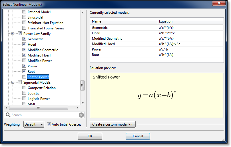
On the left side of the dialog is where the desired models can be selected. Models can either be selected individually (by clicking the checkboxes next to the model), or a family at a time (by selecting the checkbox next to the desired family). All models can be selected by clicking the “root” of the tree labeled “Nonlinear Models”.

A search field appears below the picker, so that you can filter the models to a certain specification. For example, typing “sig” in the search field will show all models that have “sig” in their name, or belong to a family with “sig” in its name. The search field allows you to quickly find a desired model in the hierarchy.

For convenience, the list of currently selected models will appear in the Currently Selected Models list in the upper right region of the picker. A preview of the equation for the currently pointed-to model is rendered in the Equation preview region in the bottom right area of the picker.

The Automatic Initial Guesses checkbox allows you to enable or disable automatic initial guessing for the calculation of the selected nonlinear models. If this box is enabled, CurveExpert Professional will provide high-quality initial guesses for built-in models, and for custom models, the custom model initialization (if any) will be called. If this box is disabled, you will be prompted for initial guesses for every model selected.

Note

if automatic initial guesses are disabled, the multicore capability, if enabled, will not be used for the currently selected batch of models.

Creating a Custom Model¶

The nonlinear model picker also provides for a quick way of creating a custom model (normally, custom models are created with Tools->Custom Models, see Creating Custom Models and Functions). To utilize this feature, simply click on the Create a Custom Model expander. This will open a small area in which you can type the name and equation for a model, and save it. Upon saving, the new custom model will be immediately available in the left pane for selecting.

Setting the Weighting Scheme¶

To set the weighting scheme desired for the models that are to be computed, select the weighting scheme from the chooser at the bottom left of the dialog. See Weighting for further details on the weighting schemes.

Manually setting initial guesses¶

Two situations cause the manual initial guess window to appear; one is if you choose to disable automatic initial guesses in the nonlinear model picker. The other is if a nonlinear regression fails, and you choose to set the initial guesses yourself in an effort to successfully calculate that model.

The manual initial guess window is shown below:

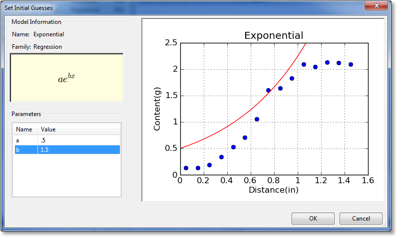
For informational purposes, the name, family, and equation for the nonlinear regression is shown in the upper left quadrant of the window. The parameters can be adjusted in the bottom left quadrant by clicking on the entries. As you adjust parameters, the graph drawn on the right will adjust accordingly. This gives real-time feedback on the parameter adjustment so that you can quickly refine the initial guesses into a reasonable state.

Smoothing¶

Introduction¶

Smoothings generate a new set of data points from the existing dataset. In CurveExpert Pro, Lowess smoothing is supported, as well as moving averages with an averaging window defined by the user.

Lowess Smoothing¶

To calculate a Lowess smoothing, select Calculate->Lowess Smoothing from the main menu. Lowess smoothing (which stands for LOcally WEighted Scatterplot Smoothing) builds on regular linear regression in order to smooth an existing dataset; in this context, an entirely new dataset will be generated that represents the smoothed data. Lowess smoothing generates a polynomial fit to a subset of data around each point in the dataset. More weighting is given to points near the point of interest, and less weight is given to points far away. After the polynomial is determined, a “smoothed” y data value is obtain by evaluating the polynomial at x.

The weighting function used is the tri-cube weighting function for $|x| < 1$ :

$w(x) = \left (1 - |x|^3 \right )^3$

where $x=(x_i - x_p)/s$ , and the weighting function is zero for $|x| >= 1$ . $x_p$ is the point of interest, and $s$ is the maximum distance of any point in the local dataset to $x_p$ .

The polynomial used by CurveExpert Pro is a simple degree-one linear regression. Once the smoothed values are obtained, a linear spline is used to connect the points for visualization and evaluation purposes.

Note

William S. Cleveland: “Robust locally weighted regression and smoothing scatterplots”, Journal of the American Statistical Association, December 1979, volume 74, number 368, pp. 829-836.

Note

William S. Cleveland and Susan J. Devlin: “Locally weighted regression: An approach to regression analysis by local fitting”, Journal of the American Statistical Association, September 1988, volume 83, number 403, pp. 596-610.

Savitzky-Golay Smoothing¶

To calculate a Savitzky-Golay smoothing, select Calculate->Savitzky-Golay Smoothing from the main menu. Savitzky-Golay (SG) smoothing combines a moving-average-type averaging with a locally-fitted polynomial in order to smooth an existing dataset. The user has the opportunity to select the number of points in the moving average window (the number of points must be odd), and the degree of the polynomial used to fit the data within each window. Additionally, the degree of the The input dialog for the SG parameters is shown below.

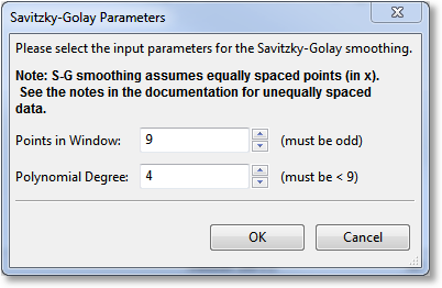
SG smoothing is primarily intended for data that is equally spaced in x (typically, x is time). In cases where the x data is not equally spaced, CurveExpert Pro still assumes that it is for the purposes of performing the smoothing. Doing so virtually shifts the data points to equally spaced positions within the averaging window. In cases where smoothing is useful in general, this shift is the equivalent of introducing an additional source of noise in the function values; however, this noise will often be much smaller than the noise already present in the samples. Thus, the smoothing is still useful, but should be used with care. The nature of smoothing in general is just to guide the eye through a forest of points, so the user can determine if the output smoothing performs its desired task rather easily.

Moving Averages¶

Moving average applies an averaging window to each point in a dataset, in turn, in order to generate a new set of data. The size and type of window determine the amount of averaging that will take place. To calculate a moving average, select Calculate->Moving Average from the main menu. A dialog will appear that will allow you to select the window to utilize for the averaging.

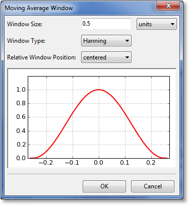
The first parameter to select for the window is its size. Here, you can select the size (sometimes called the extent) of the window in terms of units (meaning a distance along the x axis), or in terms of number of points. The (0.0) location on the preview is always defined to be at the x location of the point being window averaged. The window preview will continually update in order to show the currently defined window. Note that the underlying dataset must be sorted in order for the window to be specified in terms of a number of points. If the dataset is not sorted, the points choice is disabled.

The window type can also be selected from the following:

rectangular
Bartlett (triangular)
Blackman
Hamming
Hanning

The window type affects the weighting factor that is applied to each point within the window that is to be averaged. For example, a rectangular window applies a weight of 1 to all points within the window.

Finally, the relative window position can be set. Usually, a centered window is used, which places the center of the window at the same x location as the data point being averaged (location 0.0). Alternatively, you can select a leading or lagging window, which places the window ahead of the data point or behind the data point, respectively.

After tuning the window parameters to the desired settings, click “OK”, and the moving average will compute and display.

Functions¶

Introduction¶

Functions in CurveExpert Professional depend on the independent variables (x) only, with no free parameters. Functions are available in CurveExpert Pro for convenience, and you can perform all of the normal operations on functions that you can on any other results.

To calculate a function, select Calculate->Functions from the main menu. There does not have to be a dataset present in order to compute a function.

Note

Selecting a Function or Functions¶

Upon selecting Calculate->Functions, the function picker will appear; all functions appear in this picker (built-in functions and custom functions) that are appropriate for the number of independent variables in the dataset. A screenshot of the function picker is below:

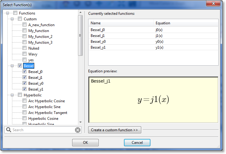
On the left side of the dialog is where the desired functions can be selected. Functions can either be selected individually (by clicking the checkboxes next to the model), or a family at a time (by selecting the checkbox next to the desired family). All functions can be selected by clicking the ‘root’ of the tree labeled ‘Functions’.

A search field appears below the picker, so that you can filter the functions to a certain specification. For example, typing “bes” in the search field will show all functions that have “bes” in their name, or belong to a family with “bes” in its name. The search field allows you to quickly find a desired function in the hierarchy.

For convenience, the list of currently selected functions will appear in the Currently Selected Functions list in the upper right region of the picker. A preview of the equation for the currently pointed-to function is rendered in the Equation preview region in the bottom right area of the picker.

Creating a Custom Function¶

The function picker also provides for a quick way of creating a custom function (normally, custom functions are created with Tools->Custom Functions, see Creating Custom Models and Functions). To utilize this feature, simply click on the Create a Custom Function expander. This will open a small area in which you can type the name and equation for a function, and save it. Upon saving, the new custom function will be immediately available in the left pane for selecting.