Digitizing

Introduction

In some cases, the data to be analyzed is in the form of a picture or image. In CurveExpert Professional, you can use the built-in digitization capabilities in order to extract the data present on an image into a dataset (to “digitize”, in this context, means to convert content from an image into a usable dataset). To successfully digitize information from an image into data, information about how pixels in an image map to real data must be collected by the application, and the digitizer leads you through this process.

The digitizer supports Cartesian (XY) and polar plots; XY plots can have semilog or log-log axes. Skewed axes are also supported intrinsically by the transformations performed by the digitizer engine.

In order to invoke the digitizer, choose Data->Digitize from image from the main toolbar. This will begin the digitization process; first, you will be able to select the image, and then the dialog leads you through the digitization steps as documented in the following sections. In general, there are three primary steps to creating a successful digitization: * select the image * calibrate * select data points Selecting the image is straightforward; the image can either be read from a file on disk, or pasted from the clipboard. Calibration is the means by which you describe where the axes of the plot are located, and how those axes map to real numbers. Selecting of the data points tells the digitizer which locations you would like to have digitized into data.

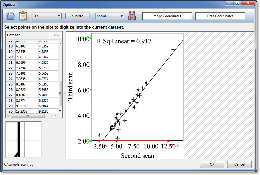
The layout of the digitizer dialog is shown below:

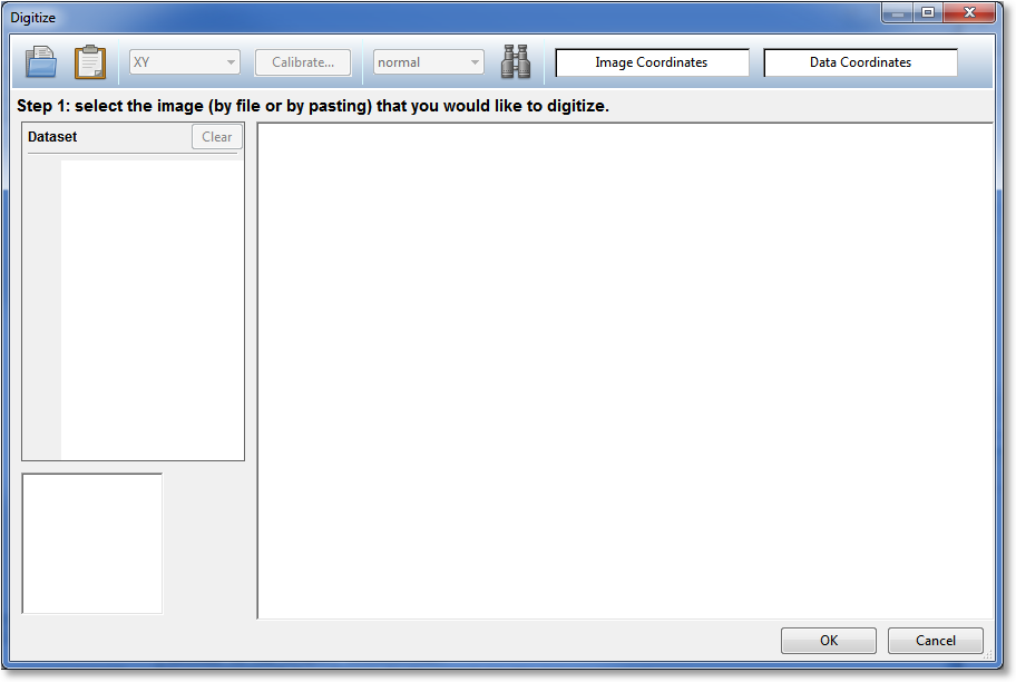
The toolbar is shown across the top, with the appropriate buttons only being enabled at the appropriate times as you move through the digitization process. Beneath the toolbar, an informational message will appear that is intended to remind you what you are working on in the digitizing process. The data values that have been digitized so far are shown in the “Dataset” section. The image, current calibration, and currently selected points are shown in the canvas area in the bottom right. The bottom left area is a magnifier, where the contents of the image and overlay underneath the mouse crosshairs are magnified by a factor of 2X of the 100% image size. Finally, the path to the currently selected image is shown along the bottom of the window, to the left of the OK and Cancel buttons.

To exit the digitizer and save the current dataset, click OK; to exit the digitizer while discarding your current work on the dataset, click Cancel.

Step 1: Select the image

First, the image can either be read from a file, or pasted from the clipboard. To read from file, click the first button in the toolbar, and select your file. Supported file formats are PNG, BMP, JPEG, GIF, PCX, PPM, TGA, TIFF, WMF, XBM, XPM, and Photoshop 2.0/3.0 PSD files. If the image on the clipboard is desired, either click the Paste icon in the toolbar, or right-click the image and select Paste Image.

Note that once the image is imported into the digitizer, the file that it was imported from (if it was not pasted) does not need to remain on disk. The image data will be saved as part of the digitizer, and is also persistent in the CurveExpert Professional document.

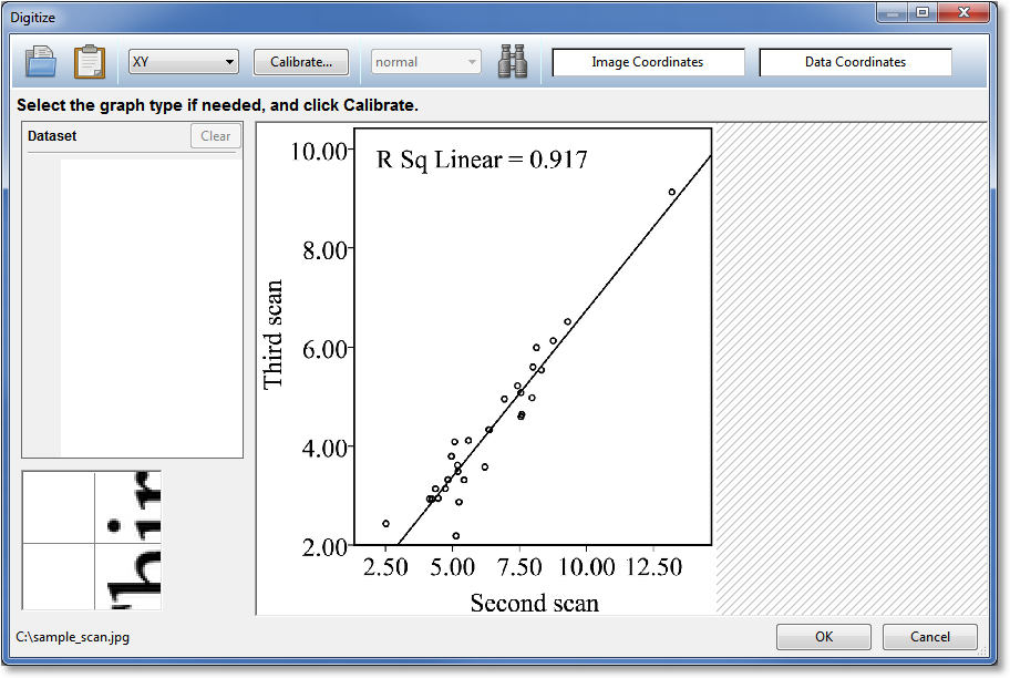
Step 2: Calibrate

Once the image is in place, you may select the type of the graph in the image from the toolbar. Most commonly, plots are simple XY plots with linear x and y axes. However, CurveExpert Professional supports digitizing from XY plots with the x and/or y axis on a log scale, and also supports Polar plots.

The calibration may now be performed. Click the Calibrate… button, and follow the prompts that are given beneath the toolbar. For an XY plot, you will first click on the leftmost tick mark possible on the x axis, and then click on the rightmost tick mark possible on the x axis. You will soon be asked which data values (in the x direction) these two tick marks correspond to. Also note that you can fine-tune the location of the point you chose by hovering the mouse over the red dot that you just created, and using the keyboard arrows to shift the dot until it adequately lines up with both the axis and tick mark. Use the magnifier to aid in this fine tuning. A red dot will be placed to indicate each of your calibration points, connected by a red line. The canvas will look similar to the screenshot below.

Note

You may fine-tune the calibration points at a later time as well.

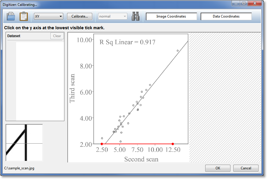
After specifying the X axis calibration, we will now specify the calibration for the Y axis. In the same manner as the X axis was calibrated, click on the Y axis at the lowest possible tick mark on the Y axis, and then at the highest possible tick mark on the Y axis. The Y axis calibration points will be indicated by green points connected with a green line.

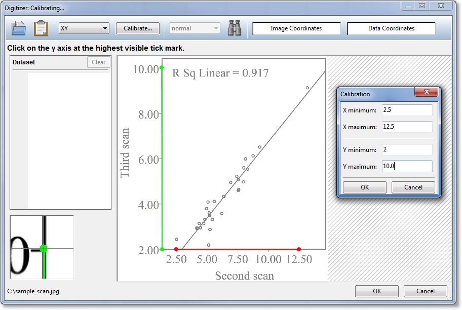
Once the second Y calibration point is selected, the calibration dialog will appear to allow you to input the data values that corresponding to each of the calibration points; this is shown in the screenshot below. For XY plots, you will specify the data values for the two points selected on the X axis, and then for the two points selected on the Y axis. After filling in this information, your calibration data values will display in red or green next to the calibration points in the image.

Remember that you can still fine-tune the location of the calibration points by pointing at them with the mouse and using the arrow keys to move the calibration point to the desired location. Any data points that you have already created will be automatically adjusted as the calibration changes.

Also, if you desire to replace the current calibration with a completely new one (as opposed to fine-tuning the existing calibration), simply click the Calibrate… button again.

As you move the mouse over the image, you will notice that the Image Coordinates and Data Coordinates information bars will begin to show information concerning the current mouse location. The image coordinate is the pixel location within the image. The data coordinate is the transformed data value subject to the current calibration (i.e., the mapping between coordinates in the image and the real data coordinates).

Calibrating polar plots

The procedure for calibrating polar plots is slightly different than XY style plots; in the case of a polar plot, you will only be asked to click on the center of the polar plot, and also to click on the zero-degree axis at the tick farthest from the center. The line formed by these two points define the angle on the image that corresponds to zero degrees, and you provide the two data values (radii, in this case) that correspond to the two clicked points. The calibration dialog will query you for the Rmin and Rmax values.

Step 3: Select data points

Now that the calibration is in place, click on the image to create data points where desired. The most common method is to simply click on the middle of each data point. As you click on the image to create data points, the points are both displayed on the image as a ‘+’ marker, and the data values show in the area of the dialog as well. Like calibration points, you can fine-tune a point’s exact location in the image by pointing at its marker in the image (it will turn magenta when active), and using the keyboard arrows. The fine-tuning arrows also work immediately after the mouse click that creates the marker.

As the mouse passes over a marker, both the marker and its corresponding data value in the dataset are highlighted in magenta.

To delete an existing marker (and by extension the data value), point at it with the mouse, and press the Del key.

If in polar mode, the X value (first column) in the dataset is filled in with the angle in degrees, and the Y value (second column) in the data set is populated with the distance from center corresponding to your Rmin/Rmax calibration.

Point autodetection

In some cases, there are too many data points to manually pick, in these cases, the point autodetection should be utilized. There are two controls in the digitizer toolbar that control how autodetection behaves: the sensitivity setting (normal, aggressive, or conservative), and the autodetect button.

The idea behind the point autodetection is that you provide the digitizer with a small piece of the image that represents the data point (called the template), and then the digitizer searches the image for other instances of that template in the image. Therefore, you will want to provide a data point marker that is well separated from any other elements in the image, such as background text, axes, other data markers, or curves. Also, it helps for accurate selection to maximize the digitizer window (in order to maximize the size of the image canvas), or right-click the image canvas and select a larger zoom value.

During the point autodetection, the toolbar will turn red.

To provide the data point marker template, click the autodetect button on the toolbar. Draw a box around a data point marker, and as soon as the box is finished, the digitizer will start the computation to detect other similar data point markers in the image. These will be marked with a ‘+’ overlay marker just as if you selected them yourself. For best results, try to draw a box tightly around the marker, such that the marker is centered in the box.

Inevitably, the automatically detected markers need to be cleaned up. At this time, you can clean up the results by pointing at markers that aren’t quite right, and using the arrow keys to fine tune them. Markers that are missed can be added simply by clicking on the marker. Markers that are completely incorrect can be selected by pointing at them, and pressing the Del key.

Step 4: Complete the digitization

Simply press OK in order to import the digitization results into the CurveExpert Professional spreadsheet. At any time, you can modify the digitization by again selecting Data->Digitize from image and modifying your existing digitization of the image.

Using the image canvas

The image canvas is the primary means by which interaction takes place to define the digitization. You will use the canvas to select points for calibration, pick points for digitization, and interact with those points.

The image is displayed in “Fit to Window” mode by default. In this mode, you will always be able to see the entire image; however, since it is resized to fit the window, the image quality will not be optimal. Use of the magnifier at the bottom left mostly mitigates this shortcoming.

In order to view the image at fixed magnification settings, right click the image canvas and select the desired magnification of 50%, 100%, or 200%. A magnification of 100% shows the image at its native resolution, pixel-for-pixel.

As mentioned several times above, the calibration settings are shown in red and green, overlaying the base image being digitized. Digitized data points are shown with a plus (‘+’) marker. You may delete a marker by pointing at it and pressing the Del key. Fine-tuning a marker is performed by pointing at a marker, and pressing the arrow keys on the keyboard to move the marker into the desired position.