Creating Custom Models and Functions

Introduction

CurveExpert Professional allows very powerful construction of custom models and custom functions. By way of reminder, a “model” in CurveExpert is used to calculate nonlinear regressions, and are dependent on both the indepedent variables (x) and a vector of parameters (a). A “function” is a dependent on the independent variables only.

Creating your custom models/functions can be performed with the choices under the Tools menu; there are two classes of interfaces: simple interface, and advanced interface. For most needs, the simple interface suffices, as it allows the user to express a model in a one-line expression form.

Note that you can create custom models and functions at any time; they are saved so that you can use them when you compute nonlinear regressions or functions later, and they appear in the “Custom” part of the nonlinear regression picker (or function picker) when you choose Calculate->Nonlinear Model Fit or Calculate->Function.

Custom Models

To create a custom model, select Tools->Custom Models. This will show the model manager, which allows you to delete or save custom models.

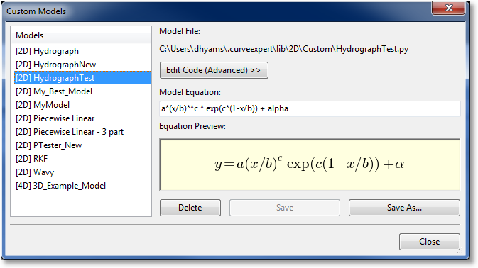
To get started, simply type the expression for your model into the “Model Equation” field. Do not include “y = ” as a part of your equation; just the expression will suffice.

As you type, CurveExpert Professional will guess how to render your equation, even converting Greek letters into the appropriate representation. The Equation Preview (see Equation Display) shows how your equation will render in CurveExpert. Note that its guess is not adjustable in the simple interface; if the rendering is undesirable, it can be adjusted by editing “latexequation” attribute for the model directly by clicking the “Edit Code (Advanced)” button. See Custom Models: Advanced Usage for more details. Usually the equation rendering is reasonable and correct, but in those cases in which it is not, remember that the rendering does not matter as far as the calculation and mathematics are concerned.

Once your model is written the way that you like, simply hit the Save or Save As button, depending your intent. Give your model a name, and your model will then appear in the list on the left, signifying that it is now available for use within CurveExpert Professional, when you choose to compute nonlinear regressions.

Mathematical Operations

Obviously, the standard arithmetic operations are supported. Multiplication is performed with a *, division with /, addition with +, and subtraction with -. Raising a quantity to a power is performed with either ^ or **, with the ** notation being preferred. Grouping is performed with parentheses ().

Reserved Words

In any model, the independent variable is always denoted by x. If you are writing a model that is a function of multiple independent variables, these are denoted as x1, x2, x3, and so on. Each of these special variables are reserved words and should not be used as a parameter name in your model.

All mathematical functions supported by CurveExpert Professional, such as sin, cos, tan, exp, etc., are also reserved words. See Appendix A: Math Functions for a complete list of the mathematical functions supported.

Any other name that CurveExpert Professional sees in your model is treated as a parameter. This powerful feature lets you name your parameters any name that you find appropriate, such that the model’s syntax carries meaning. Thus, names such as beta, my_long_parameter_name, and b are all legal parameter names. Note also that names are case sensitive; the parameter a is distinct from the parameter A, for example.

Custom Functions

Custom functions are exactly like custom models, but without any parameters; they are only dependent on the independent variable(s). As such, if you enter a custom function, CurveExpert will flag any unknown name in your equation as an error. Also, custom functions have a default domain setting that can be set to assist the autoscaler, as documented in Autoscaling. Otherwise, creating a custom function is exactly the same as creating a custom model, which is documented above.

Custom Models: Advanced Usage

If your needs for a model are more complex than a one-line equation, CurveExpert Professional has the capability of allowing you to program a model as complicated as you like. This capability is accessible via the Tools->Custom Models menu choice; then, click “Edit Code” to directly access the code that implements the model.

Rather than trying to reinvent another language for the user to express a model in, CurveExpert uses Python as its base model language. Thus, anything that can be done in Python can be done in your custom models. This gives the user extreme flexibility in the custom models, even to do things like download data from a web server that influences how the model is computed. Here, your creativity is the only limit.

Documenting the entire Python language and its capabilities are obviously outside the scope of this document; for this, refer to http://docs.python.org/release/2.6.6. You do not, however, need to be proficient in Python to be reasonably productive directly editing a custom model. Just follow the examples given as a part of CurveExpert Professional, and for further reference, look in the “lib” and “libf” directories in the core CurveExpert Professional distribution (where the program files are located; see Where files are located). These directories contain all of the CurveExpert Professional built-in models and built-in functions.

Note

Python uses indentation to identify code blocks (for example, the code that should execute when an if statement is true). So, if you have an unexplainable syntax error in your model, make sure that your indentation is correct.

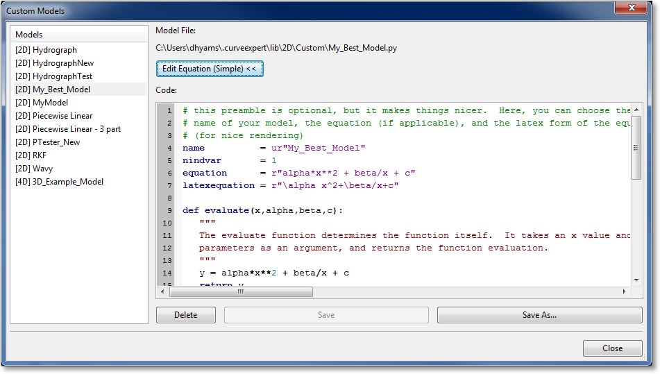
Upon selecting the “Edit Code” button, the dialog expands, and the coding window replaces the simpler interface where you can just enter the equation directly (to return to the simpler one-line equation editing, just press Edit Equation). The coding window has full syntax-highlighting capability, and you can use standard cut/paste shortcuts ink the window in order to facilitate code construction.

Note

If you have an error in your custom model, it will have [ERROR] appended to its name for identification. To correct it, simply select it and edit the code in the coding window.

Remember also that you can view the code for your simple models through this interface, to view what is going on “behind the scenes”, as well as to adjust easy things like the latexequation, in case you want to change how your model equation is rendered. In fact, when you create a model in the simple interface (one-line equation), CurveExpert Professional just writes the Python code on your behalf.

As in regular Python, any characters following a # sign are a comment, and are highlighted in green in the coding window.

Every model should have at least four items (name, nindvar, equation, evaluate), with the other two items (latexequation and initialize) being optional.

name

This is a variable to define the name of your model, which is the name used throughout CurveExpert Professional to refer to it. The name of your model is also used to generate the filename in which it is saved, the full path of which is shown above the coding window. The type of this variable is a string, and should be enclosed in quotes.

nindvar

This is a variable to define the number of independent variables that this model expects. Most of the time, this value will be 1, but can obviously be higher depending on how many independent variables you want your model to apply to.

equation

This is a variable that is a text representation of the equation. It is for information only, and is displayed by CurveExpert Professional in different areas of the software.

latexequation

This is a variable that is a mathtext representation of the equation (see Mathtext and Appendix B: Math Symbol Reference for how to write in mathtext). In short, this is a TeX-like version of your equation that will be used every time rendering of your equation is required in CurveExpert Professional. This variable is optional, and if not present, CurveExpert Professional will attempt to guess it by looking at the “equation” variable above.

evaluate(x,a,b,c,d,...)

This is the most important part of your model; evaluate() is a function that is called whenever your model is evaluated with the independent variables and a set of parameters. It is this function that is called in the course of the parameter optimization process, and it is called in order to draw your plot.

The evaluate function must take x as its first argument. This x is the vector of independent variables, and can be multiple columns if there is more than one independent variable. Following x is a comma separated list of parameters, which can have any name. The job of the evaluation function is to take these pieces of data and compute an output vector y, returning it as the result of the evaluation.

An example of an evaluate function is the following (with comments removed for brevity):

def evaluate(x,a,b,c):
    return exp(a + b/x + c*log(x))

Any other Python function (denoted by the def keyword) other than evaluate and initialize are ignored. This means that you can create your own Python functions and call them from your evaluate function as you wish.

initialize(x,y)

The initialize function is optional, but can greatly aid in the convergence of a model’s parameters in the process of nonlinear regression. initialize() is a function that takes the independent variables as the first argument, and the dependent variables as the second (both of these quantities are based on the data currently held in the spreadsheet). With this data, you can perform any analysis necessary to compute good initial guess parameters to start with. The parameters can be returned as anything that can be translated into a Python array, but most commonly are returned simply as a comma separated list.

Good examples of using initialize() can be found in CurveExpert Professional’s built-in models, by way of example (the built-in models are located in the “lib” directory where the program files are; see Where files are located). A common approach there is to transform the model into a linear one, solve a linear least squares system, and use the output from that in order to initialization the nonlinear regression.

An example of an initialize function is the following (with comments removed for brevity):

def initialize(x,y):
   try:
       n = len(x)
       A = ones((n,3))
       A[:,1] = 1.0/x
       A[:,2] = log(x)
       B = log(y)*log(x)
       soln,residues,rank,s = lstsq_solve(A,B)
       a,b,c = soln  # use Python's unpacking to extract a,b,c from the solution
   except:
       a,b,c = 1.0,1.0,1.0

   return a,b,c

In this case, an attempt is made to transform the model into a linear least squares system and a solve of that system is tried. If that fails (for example, if there is a zero in the data, the last two columns of A cannot be computed), the solution is just initialized to three ones.

Custom Functions: Advanced Usage

Again, custom functions are the same as custom models except that they have no free parameters. The evaluate() function takes only x as an argument, and there is no need for an initialize() function. The advanced interface for editing and creating custom functions is otherwise exactly the same as the one for custom models described above. An example evaluate function is below:

def evaluate(x):
    return exp(x)*sin(x)

For 3D and higher functions, like custom models above, x is a multicolumn vector. To extract out each column for convenience, an example is given below:

def evaluate(x):
   x1 = x[:,0]
   x2 = x[:,1]
   return x1*sin(x2)