Calculating Results
CurveExpert Basic supports TWO distinct classes of results:
regressions
linear regressions (linear and polynomial fits)
nonlinear regressions (built-in and custom models)
interpolations
cubic spline
tension spline
Calculation of these results can be accessed through the Calculate menu in CurveExpert Basic, or optionally via the corresponding buttons on the toolbar (see Toolbar).
General Guidelines
Scaling Datasets
For best results, always scale your data sets to the order of one. You may do this prior to reading in your data file, or after your data file has been imported using the scaling feature in CurveExpert Basic (see Operating on Data).
Imagine a data set with x values ranging from 1000 to 10000 and a regression model where the term exp(a*x) is involved. Unless a very good initial guess for a is given, chances are that an exponential to a very large power (eg. exp(1000)) will be taken in the course of the nonlinear regression algorithm. The calculation will overflow, and the regression will fail as a result. Even if the regression happens not to fail, the regression algorithm will have an exceedingly tough time finding the correct parameters, since a small change in the free parameters will cause a tremendous change in the size of the term. The moral of the story: always scale your data!
As another example, if you have data that describes atmospheric pressure at different elevations, you might have (in metric units) a data set that looks like:
x=[-100, 0, 100, 500, 1000, 4000] meters
y=[102000,101325,101000,100500,100000,99900] Pascals
Using the Data->Scale feature in the Data menu of CurveExpert Basic, you can scale this data using a scale factor of 0.001 on the x data, and 0.00001 on the y data. So, you would then have the following data set:
x=[-0.1, 0, 0.1, 0.500, 1, 4] kilometers
y=[1.02,1.01325,1.01,1.005,1.0,0.999] bars
The second example is much more likely to allow nonlinear regressions to converge, and also will allow higher order polynomial fits to be performed with more accuracy. If you have a data set that seems particularly ill-behaved, scaling can help solve this problem.
Note that CurveExpert Basic is able to perform correctly on data in any scale, as long as the calculations do not overflow or underflow. So, if a data set is giving problems, scaling it should be the first action to take.
Set the tolerance parameter reasonably
Don’t set the tolerance parameter (in Edit->Preferences->Regression) too low. In regression modeling, not much advantage is to be gained by setting a very strict tolerance. Its main purpose in life is to prevent the nonlinear regression algorithm from converging on local minima, not to make the calculated parameters more accurate.
Data should be appropriate to the model
Make sure that the data is appropriate to the model. Especially look out for using logarithmic or exponential families of models with data that contains zeros or negatives. For example, it is not possible, in any shape or form, to obtain a negative or zero with the basic exponential model (y=ae^(bx), assuming a is positive; the inverse problem exists for a negative a). So, it is not wise to use a model that cannot reflect the trends in the data.
Interpolation
Introduction
An interpolation, by definition, passes through every data point, and as such, the correlation coefficient will always be 1, and the standard error will always be zero. CurveExpert Basic supports cubic splines and tension splines. All splines are defined in a piecewise fashion between data points.
Note
The dataset must be sorted (based on the independent variable) in order for any spline interpolation to work. Select Data->Sort from the main menu in order to sort your dataset if necessary. If CurveExpert Basic detects that your dataset is not sorted, it will not allow spline interpolations to be selected.
Cubic Splines
To calculate a cubic spline, select Calculate->Cubic Spline from the main menu. The cubic spline is simply a polynomial spline of order 3; cubic splines are the most common form of spline. Cubic splines guarantee continuity in the spline, and continuity in the first and second derivatives of the spline at the data points. At the endpoints, the second derivative is set to zero, which is termed a “natural” spline at the endpoints, as the curvature goes to zero.
Tension Splines
To calculate a tension spline, select Calculate->Tension Spline from the main menu. A prompt will appear to ask for the amount of tension desired. Tension splines are based on hyperbolic functions, and simulate a cord being stretched with a defined tension (amount of force) between the data points. An extremely high tension approaches a linear spline, and low tensions will appear correspondingly “loose” around the data points, resembling a cubic spline.
Linear Regression
Introduction
Linear regressions, as a class of results, can be calculated directly, and do not need an iterative process like nonlinear regressions do. See Linear Regression in the appendices for a more in-depth explanation. A linear regression can be constructed from any model that is a linear combination of functions; the coefficients in the linear combination are the parameters to be found.
There are two types of linear regressions supported in CurveExpert: linear and polynomial. All other regressions, even if they could be calculated as a linear-type regression through a variable transformation, are computed with the nonlinear regression engine.
Linear Fit
In CurveExpert Basic, you can choose to calculate a straight line regression:

by choosing Calculate->Linear Fit.
nth Order Polynomial Fit
To calculate a polynomial via linear regression, choose Calculate->nth Order Polynomial Fit. A prompt will appear to ask for the degree of polynomial desired. Also, in the same prompt, you can choose to force the polynomial through the origin, which forces the intercept to zero. Also, you may choose the desired weighting for each point in the dataset (see weighting for further information) After entering the degree (and origin forcing or weighting as appropriate), the polynomial will be computed and added to the result list.
Nonlinear Regression
Introduction
Nonlinear regressions are solved with the Marquart-Levenberg method as documented in Nonlinear Regression in the appendices. To calculate a nonlinear regression, select Calculate->Nonlinear Model Fit from the main menu.
Selecting a Model or Models
Upon selecting Calculate->Nonlinear Model Fit, the nonlinear regression picker will appear; all models appear in this picker (built-in models and custom models) that are appropriate for the number of independent variables in the dataset. A screenshot of the model picker is below:
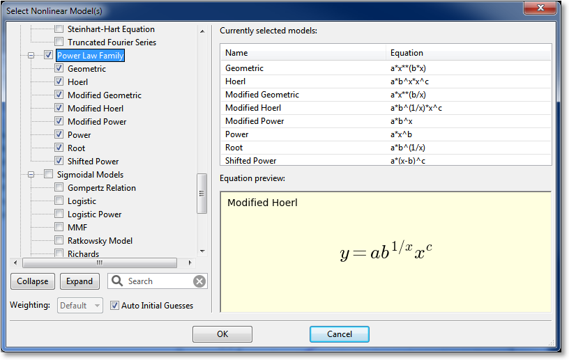
On the left side of the dialog is where the desired models can be selected. Models can either be selected individually (by clicking the checkboxes next to the model), or a family at a time (by selecting the checkbox next to the desired family). All models can be selected by clicking the “root” of the tree labeled “Nonlinear Models”.
A search field appears below the picker, so that you can filter the models to a certain specification. For example, typing “sig” in the search field will show all models that have “sig” in their name, or belong to a family with “sig” in its name. The search field allows you to quickly find a desired model in the hierarchy.
For convenience, the list of currently selected models will appear in the Currently Selected Models list in the upper right region of the picker. A preview of the equation for the currently pointed-to model is rendered in the Equation preview region in the bottom right area of the picker.
The Automatic Initial Guesses checkbox allows you to enable or disable automatic initial guessing for the calculation of the selected nonlinear models. If this box is enabled, CurveExpert Basic will provide high-quality initial guesses for built-in models, and for custom models, the custom model initialization (if any) will be called. If this box is disabled, you will be prompted for initial guesses for every model selected.
Note
if automatic initial guesses are disabled, the multicore capability, if enabled, will not be used for the currently selected batch of models.
Creating a Custom Model
The nonlinear model picker also provides for a quick way of creating a custom model (normally, custom models are created with Tools->Custom Models, see Creating Custom Models). To utilize this feature, simply click on the Create a Custom Model expander. This will open a small area in which you can type the name and equation for a model, and save it. Upon saving, the new custom model will be immediately available in the left pane for selecting.
Setting the Weighting Scheme
To set the weighting scheme desired for the models that are to be computed, select the weighting scheme from the chooser at the bottom left of the dialog. See weighting for further details on the weighting schemes.
Manually setting initial guesses
Two situations cause the manual initial guess window to appear; one is if you choose to disable automatic initial guesses in the nonlinear model picker. The other is if a nonlinear regression fails, and you choose to set the initial guesses yourself in an effort to successfully calculate that model.
The manual initial guess window is shown below:
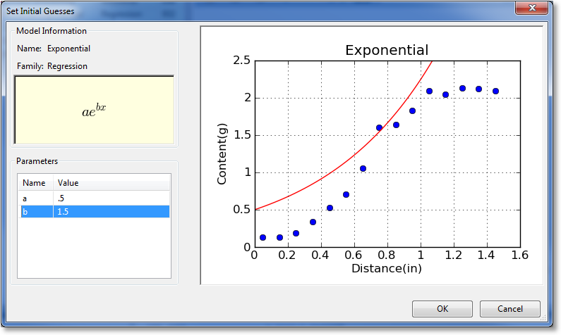
For informational purposes, the name, family, and equation for the nonlinear regression is shown in the upper left quadrant of the window. The parameters can be adjusted in the bottom left quadrant by clicking on the entries. As you adjust parameters, the graph drawn on the right will adjust accordingly. This gives real-time feedback on the parameter adjustment so that you can quickly refine the initial guesses into a reasonable state.