
All result query operations are available through the graph. Right click on the graph in order to access the query operations.
The Model Information dialog gives all of the information needed to apply a curve fit and some supplemental information about the performance of the given model. The most important information contained in this panel are the values of the parameters of the model.
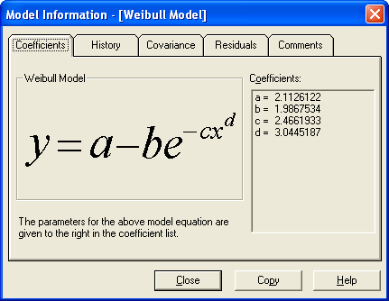
The Coefficients page gives the most vital information about the model in the current graph. The values of the coefficients are given here as well as the model equation, so that meaning of the parameters is clear.
The Model section gives the data modeling equation so that the interpretation of the coefficients is clear. The coefficients a,b,c, etc. in the Coefficients section match the corresponding parameters shown in the model.
The Coefficients section gives the values of the relevant parameters for the current model – these coefficients are always expressed as a, b, c, d, and so on. These coefficients match the model shown in the Model section. If the list of coefficients exceeds the extent of the window that they are shown in, a scrollbar will appear to allow you to scroll through the parameters.
If the Copy button is pressed when the coefficient tab is active, the list of coefficients is copied to the clipboard.
The History page shows the value of the chi-square and each parameter in the current curve fit as a function of the iteration number. These values give information on the path that the nonlinear regression algorithm took to optimize the parameters (where optimization means reducing the chi-square value as much as possible). This page is divided into two sections: the Chi-Square History, and the Parameter Histories.
The Chi-Square history section shows the iteration number in the left column, and the value of the chi square at that iteration on the right. At iteration zero, the associated chi-square is computed with the initial guesses. To view the history for any parameter, use the list box beside Param 1 or Param 2. Two lists are provided so that the user can compare changes in two parameters at once.
Note that the History page is only meaningful for nonlinear regression type curve fits. Linear regressions and interpolations can be solved directly, so there is no iteration involved in their solution.
If the Copy button is pushed when the history tab is active, the complete history for the chi-square and then each parameter is copied to the clipboard in successive columns.
The covariance matrix gives further information about the relation between the model parameters and their uncertainties. The entries along the diagonal are directly related to the uncertainty in each parameter – for example, the entry in matrix position (2,2) corresponds to the uncertainty in the second parameter (which is b). The off-diagonal components are the covariances between parameters. For example, the entry in matrix position (3,4) is the covariance between parameters 3 and 4 (which are c and d). The covariance matrix can be used in further statistical analysis of the regression model and its goodness-of-fit. At this time, CurveExpert offers this matrix as additional information to the user, and does not draw any conclusions based on its entries. Note also that the inverse of the covariance matrix is the curvature matrix.
If the Copy button is pushed when the covariance tab is active, the entire covariance matrix, in nxn format, is copied to the clipboard.
The residual plot graphically depicts the difference between the data points and the model evaluated at the data points. The residual at point i is defined by
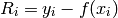
where yi is the measured value at xi, and f(xi) is the predicted value at xi. These distances are shown as bars or points on the residual plot; the magnitudes of the data points are simply replaced by the residual defined above. If the residual is positive, then the data point is above the models prediction; likewise, if the residual is negative, then the data point is below the models prediction. The residuals can provide an indication of a particular models performance. If there are runs of like-signed residuals, then a better model for the data is likely to exist.
Optimally, the residuals should exhibit a random scatter around zero, which indicates that the data points are randomly distributed around the curve. A run is a sequence of like-signed residuals, which stand out on the residual plot. A large number of runs indicates that data systematically deviates from the curve.
Press this button to open or close a large residual plot. Opening the plot simply shows the residual plot in its own window in which you may resize, zoom, print, and alter the properties just as with any other graph. While the residual plot window is open, this button will change to read Close Plot. Clicking this button will then close the large residual graph.
If the Copy button is pressed when the residual tab is active, a table of residuals is copied to the clipboard. This table is in a two-column format separated by a tab character. The first column is simply the x data, and the second column is the difference between the data point and the model evaluated at that point (yi- f(xi)).
If a copy of the plot is desired, simply open a plot window of the residuals (by clicking the Open Plot>> button and then select Copy from the graphing menu of that plot.
The comments page is meant to give additional information on the error involved in the curve fit, and also gives other miscellaneous information that could apply to your particular model.
The Error section gives you information on the curve fit performance. Two quantities are used to express the “goodness” of a particular curve fit – the correlation coefficient and the standard error of the estimate. In general, the correlation coefficient will range from 0 to 1, with a correlation coefficient of 1 being the best. In some peculiar circumstances, CurveExpert will report a correlation coefficient greater than one; this is indicative of a very poor data model. The standard error will be strictly positive, with a smaller standard error representing the better curve fit. For more information, refer to the Data Modeling with CurveExpert section.
The Comments section gives you important information about the current model, such as information regarding the characteristics of interpolation, or the performance of a nonlinear regression. For nonlinear regression, the message will inform you if the fit converged, the number of iterations required for convergence, and the tolerance imposed to determine convergence.
If the Copy button is pushed when the comments page is active, the error information and the comments section is copied to the clipboard.
The Analyze Fit feature allows easy location of x/y points, differentiation, and integration of a curve fit that has been performed. Since this feature may only be used from the graphing window (by choosing Analyze from the graphing menu or pressing Ctrl-L), all calculations will be based on the model from the invoking window.
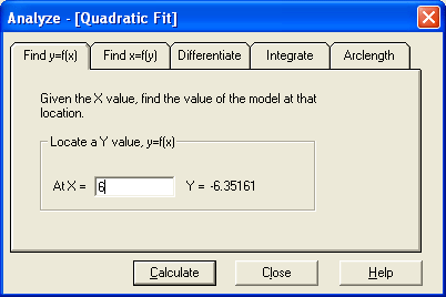
CurveExpert can evaluate the curve fit at a given x to give you the projected y value by the current curve fit. Just type in the point at which you want to evaluate the curve fit (the x value) in the “At X=” field and press Apply or <Enter> on your keyboard. The calculator will then show the corresponding y value. If CurveExpert cannot evaluate the curve fit at the point that you specified, then the word ERR is printed in the result field.
CurveExpert can evaluate the curve fit at the given y to give you the projected x value. Just type in the point at which you want the corresponding x in the “At Y=” field and press OK or <Enter> on your keyboard. The calculator will then show the corresponding x value. If CurveExpert cannot find the corresponding x value, then the word ERR is printed in the result field.
NOTE that the results obtained for the x value should be, at the least, visually checked with the graph. There is a chance the root (x-value) returned matches a y value on the graph at a location other than what was intended. This occurs simply because functions may have multiple roots, and CurveExpert may locate any one of them (since all of them are just as valid as the other) without assistance from the user. Consider a simple quadratic y=x^2: if you want the x value corresponding to y=4, there are two valid answers to this question (2 and -2). So, although this search facility in CurveExpert is very powerful, it should be used with care. The optional Initial Guess for X field should be used wisely so that the correct root is located.
Most of the time, the initial guess field is not needed; however, as mentioned above, the desired x-value may not be returned. In this case, you must set the Initial Guess for X to a value reasonably close to the root (x-value) that you are trying to find. This greatly assists CurveExpert in finding the correct root. Note that the number shown in this field when the Analyze Tool is invoked is the initial guess generated by CurveExpert, which will subsequently be used in the computation of the x-value.
Simply fill in the point at which you want to take a derivative into the “At X=” edit field. Then press the “Calculate” button, and the result will be displayed beside the “dY/dX=” entry. The default value at which the derivative will be computed is the current midpoint of the graphing window. If a derivative calculation fails, the word ERR will appear in place of the result. The derivatives are taken using a central difference combined with Richardson extrapolation to refine the derivative. This refinement is terminated when successive refinements yield less than 0.01% difference in the derivative.
To integrate a function on the interval [a,b], Fill in the value of a in the “From X=” field, and the value of b in the “to X=” field. Then press the “Calculate” button, and the result will be displayed beside the “I(ydx)=” entry. The default interval over which the integral will be taken is the current extent of the invoking graphing window. If an integral calculation fails, the word ERR will appear in place of the integral result.
The integral of the model function is taken using Simpson’s 1/3 rule coupled with the Romberg integration method. The interval is divided into successively finer subintervals which are integrated with Simpson’s rule and summed, and these results are refined with the Romberg method. Refinement is terminated when successive iterations yield less than 0.01% difference in the integral or when the interval has been divided into over 32767 subsegments. If the integral did not converge before the maximum number of segments is exceeded, a note will appear informing you of this occurrence. Use the result of an unconverged integral with due caution.
The length of the graph from point a to point b is defined as the arclength. This distance is equivalent to the distance traveled by an observer moving along the curve from the location (a, f(a)) to (b, f(b)).
Exercise caution when finding the arclength of a given plot. The formula to calculate arclength is
![L = \int_a^b \sqrt{1 + \left [ \frac{dy}{dx}\right ]^2 dx}](_images/math/f163fd8c810a71c01dd6253f7a185f0933559313.png)
So, if the derivative dy/dx becomes very small (numerically), this calculation can fail. Check your curve using the Differentiation tab to make sure that the derivative over the interval in question is not small (i.e., less than 1e-5).
The CurveExpert table generation mechanism generates a data table based on the current data model. This table will contain the calculated model values(y) corresponding to the range of x data points that you specify. To create a table, CurveExpert must know the following information:
Simply fill this information into the provided spaces on this dialog box, enter a filename, and press the ‘OK’ button. By default, the tables generated by CurveExpert have the extension ‘.TAB.’ The generated table will simply be two columns of data: the first column is the x data, and the second column is the calculated y data from the model that you specified.
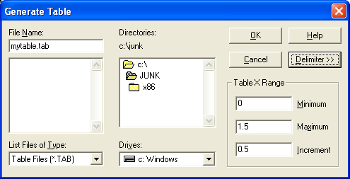
This region of the dialog box is where you can specify the starting and ending x value and the resolution of the table, as discussed above.
For example, suppose that you wanted to generate a table file named “mydata.tab” for a range of x=0.0, 0.5, 1.0, 1.5...10.0 with comma separators between columns. You would specify 0.0 in the ‘Minimum’ field, 10.0 in the ‘Maximum’ field, and 0.5 in the ‘Increment’ field. Then press the ‘Delimiter’ button and choose ‘Comma’ from the delimiter menu. Finally, you would enter the filename mydata.tab in the File Name field and press the ‘OK’ button.
Exporting a file allows you to easily transfer data out of CurveExpert, most often to a spreadsheet. The exported file will contain the data points along with the specified curve fit’s approximation to the data evaluated at every data point. Also, if you desire, the exported file can contain the specified model’s coefficients (a,b,c,d...) and statistics describing your data set such as the mean and standard deviation. The filename for the exported file is entered in the File Name field as usual. The extra buttons on the right hand side of the Export dialog are special settings for the exporting operation.
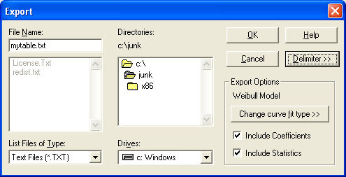
The Delimiter button allows you to choose what type of delimiter you would like to use to separate the data columns. The default is a tab delimiter, but you may also use a single space or a comma.
The curve fit that you will export is, by default, set to the last curve fit that was performed. Its name is shown in the Export Options group. If you wish to change this curve fit, click the Change Curvefit Type>> button – a list of curve fits that have already been calculated will appear, and you may select from that list. Note that a curve fit must already be calculated to be valid for exporting. If the curve fit you desire is not on the list, cancel the Export dialog, calculate the curve fit via the Apply Fit or Interpolation menus, and then reopen the Export dialog.
The checkbutton Include Coefficients signifies whether you would like the curve fit coefficients to be present in the exported file. Note that for spline interpolations, the coefficients are given as the coefficients of EACH piecewise polynomial used between each knot/data point. The default is ON.
Lastly, the checkbutton Include Statistics signifies whether you would like relevant statistics to be present in the exported file. The statistics that will be included are: X and Y data minimum, X and Y data maximum, X and Y data mean, and the X and Y data standard deviation. The default is ON.